34.3 Theoretical Bounds on Sorting

What is the best time we can get for sorting?

So far, the fastest sorts we have gone over have had $\Theta(N*logN)$as the worse case time. This begs the question; can we get a sorting algorithm that would have a better asymptotic analysis?

Let's say that we have "the algorithm ultimate comparison sort" known as TUCS which is the fastest possible comparison sort. We don't know the details of this yet-to-be-discovered algorithm as it has not been discovered yet. Let's additionally say that $R(N)$is the worst-case runtime of TUCS and give ourselves the challenge of finding the best $\Theta$ and $O$ bounds for $R(N)$. (This might seem a little odd since we really don't know the details of it, but we can find $R(N)$).

As a starting point, we can go ahead and have the $O$ bound of $R(N)$ be $O(N*logN)$. Why? If this is the fastest sorting algorithm it must be at least just as good as the algorithms we already have! Thus it must at least be as good as Mergesort's worst case as otherwise we would have a contradiction in calling this algorithm TUCS.

What about the starting point for the $\Omega$ bound of $R(N)$? Since we don't quite know any details about it we can start by giving it the best possible runtime of $\Omega(1)$. But can we make this tighter?

It turns out we can as if the algorithm sorts all of N elements, it must have gone through all of the N elements at some point of sorting it. Thus, we can arrive at a tighter bound of $\Omega(N)$. But can we make it tighter? The answer is yes, but to see the argument for why we have to consider the following game.

A Game of Cat and Mouse (and Dog)

Let's say we place Tom the Cat, Jerry the Mouse, and Spike the Dog in opaque soundproof boxes labeled A, B, and C. We want to figure out which is which using a scale.

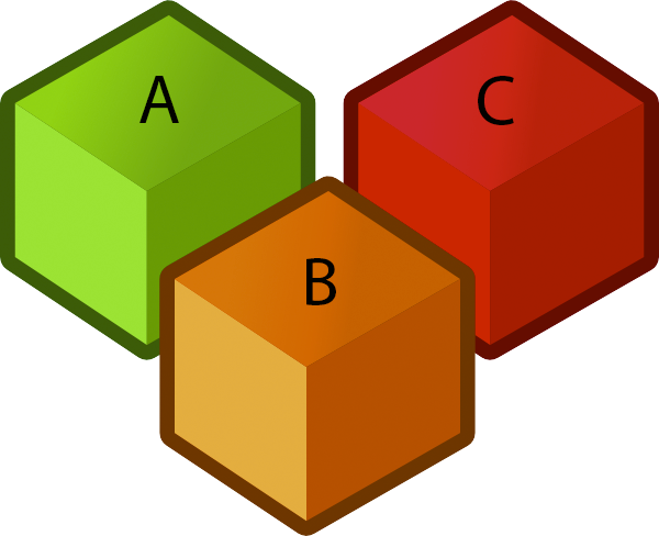
Let's say we knew that Box A weighs less than Box B, and that Box B weighs less than Box C. Could we tell which is which?

The answer turns out to be yes!

We can find a sorted order by just considering these two inequalities. What if Box A weighs more than Box B, and that Box B weighs more than Box C? Could we still find out which is which?

The answer turns out to be yes! So far, we have been able to solve this game with just two inequalities! Let's go ahead and try a third case scenario. Could we know which is which if Box A weighs less than Box B, but Box B weighs more than Box C?

The answer turns out to be no. It turns out to have two possible orderings:

• a: mouse, c: cat, b: dog (sorted order: acb)

• c: mouse, a: cat, b: dog (sorted order: cab)

So while we were on a really great streak of solving the game with only two inequalities, we will need a third to solve all possibilities of the game. If we add the inequality a < c then this problem goes away and becomes solvable.

Now that we've created this table, we can create a tree to help us solve this sorting game of cat and mouse (and dog).

But how can we make this generalizable for all sorting? We know that each leaf in this tree is a unique possible answer to how boxes should be sorted. So the number of ways the boxes can be sorted should turn out to be the number of leaves in the tree. That then begs the question of how many ways can N boxes be sorted? The answer turns out to be $N!$ ways as there are $N!$ permutations of a given set of elements.

So how many questions do we need to ask in order to know how to sort the boxes? We would need to find the number of levels we must go through to get our answer in the leaf. Since it's a binary tree the minimum amount levels turn out $lg(N!)$levels to reach a leaf. (Note that $lg$ means (log base 2)).

So, using this game we have found that we must ask at least $lg(N!)$ questions about inequalities to find a proper way to sort it. Thus our lower bound for $R(N)$ is $\Omega(lg(N!))$.