17.3 B-Tree Operations
Last updated
Last updated
The average height and depth of a BST are important properties in determining performance. Height refers to the depth of the deepest leaf and is a tree-wide property, whereas depth refers to the distance from the root of a particular node and is node-specific.
The average depth of a tree is the mean of the depth of every node.
Height and average depth determine the runtime of BST operations. The height determines the worst-case runtime to fine a node, while the average depth determines the average-case runtime of search operations.
The order in which we insert nodes has a major impact on the height and average depth of a BST. For example, consider inserting nodes 1, 2, 3, 4, 5, 6, 7
. This results in a spindly BST with height 6 and average depth 3. If we insert the same nodes in the order 4, 2, 1, 3, 6, 5, 7
, we get a much better height of 2 and an average depth of 1.43.
In considering how BSTs operate in real-life applications, we may want to start by considering randomized BSTs.
However, it is not always possible to randomize the order of insertions. For example, if we have real-time data that comes in sequentially, there is no way to shuffle the data since we do not have all the points at once.
As such, we need a different way to maintain "bushiness" in our search trees.
If we could simply avoid adding new leaves in our BST, the height would never increase. Such an idea, however, would be infeasible, since we do need to insert values at some point.
One idea that we might approach is that of "overstuffing" the leaf nodes. Instead of adding a new node upon insertion, we simply stack the new value into an existing leaf node at the appropriate location.
However, a clear problem with this approach is that it results in large leaf nodes that basically become a list of values, going back to the problem of linear search.
To ameliorate the issue of overly stuffed leaf nodes, we may consider "moving up" a value when a leaf node reaches a certain number of values.
However, this runs into the issue that our binary search property is no longer preserved--16
is to the right of 17
. As such, we need a second fix:
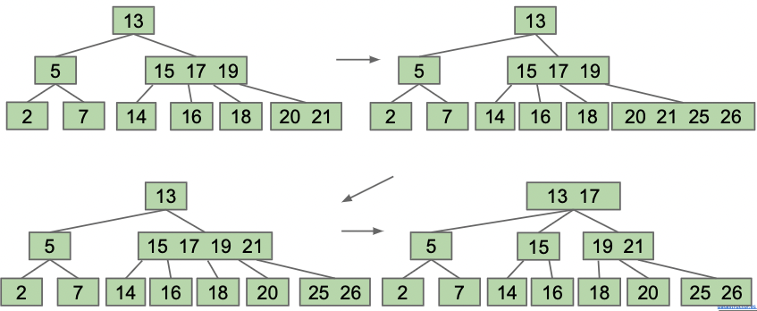
Adding to a node may cause a cascading chain reaction, as shown in the image below where we add 25
and 26
.
In the case when our root is above the limit, we are forced to increase the tree height.
Observe that our new splitting-tree data structure has perfect balance.
If we split the root, every node is pushed down by one level. If we split a leaf or internal node, the height does not change. There is never a change that results in imbalance.
The real name for this data structure is a B-Tree. B-Trees with a limit of 3 items per node are also called 2-3-4 trees or 2-4 trees (a node can have 2, 3, or 4 children). Setting a limit of 2 items per node results in a 2-3 tree.
B-Trees are used mostly in two specific contexts: first, with a small L for conceptually balancing search trees, or secondly, with L in the thousands for databases and filesystems with large records.
Luckily, on average, randomly generated insertion orders have height and average depth. In fact, you can prove that and (such a proof is beyond the scope of this course). Such properties hold even when considering both insertion and deletion.
Above, we split the children of an overstuffed node into ranges: , , and . A search on this structure would operate exactly the same as a BST, except for a value between 15 and 17, we go to the middle child instead of the left or right.
If we set some constant as a limit on our node size, our search time only increases by a constant factor (in other words, there is no asymptotic change).